Riemann curvature tensor
Motivation
(see my own answer in math.stackexchange)
In a surface we compute holonomy by parallel transporting a vector around a loop $L$ and measuring the angle change. This angle does not depends on the chosen vector to be transported. When we shrink the loop we obtain Gaussian curvature as the holonomy per unit area.
Given a pseudo-Riemannian manifold $(M,g)$,we can consider the induced parallel transport and imitate the construction above. For example, we can try with a parallelogram $L$, instead of a general loop, generated by two vectors $u$ and $v$. (Keep an eye: we are not explaining how to construct that parallelogram)
A first problem arises by the fact that the parallelogram fails to close (it has to do with Lie bracket). But suppose we know how to close the gap.
The other difference is that we can choose different vectors to transport, obtaining different values. In @needham2021visual it is defined the vector holonomy $\delta w_{\|}$ as the difference between the original vector $w_0$ and the parallel transported vector $w_{\|}$ along the "quasi-parallelogram" $L$. The length of this vector is the Riemann curvature operator.
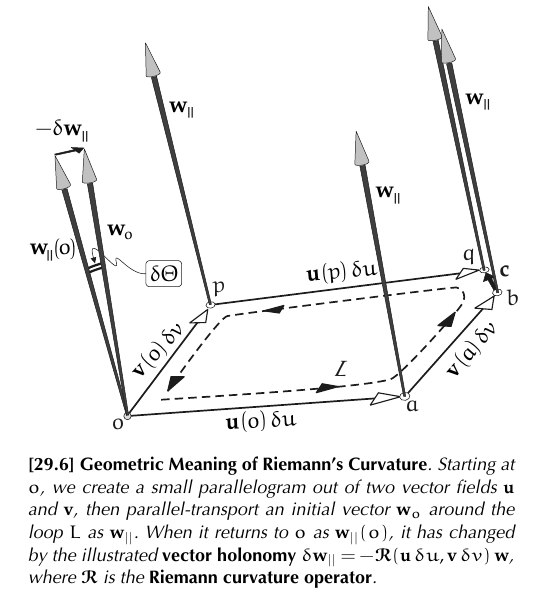
I think it should be denoted $\mathcal{R}(\mathbf{u} \delta u, \mathbf{v} \delta v)(\mathbf{w}):=-\delta \mathbf{w}_{\|}$, since it is an operator.
We can "see" it like a generalization of Gaussian curvature, since as $w$ is a unit vector, $\delta \Theta=|\delta w_{\|}|$ (a "scalar" holonomy like for surfaces), so
$$ \mathcal{K}(\mathbf{u}, \mathbf{v} ; \mathbf{w}) \asymp \frac{\delta \Theta}{\delta \mathcal{A}} \asymp \frac{\left|\delta \mathbf{w}_{\|}\right|}{\delta \mathcal{A}} \asymp|\mathcal{R}(\mathbf{u}, \mathbf{v})( \mathbf{w})| $$See @needham2021visual page 287.
It can be shown (@needham2021visual page 290), that this ideas justifies the following
Definition
The Riemann curvature endomorphism is the map
$$ R:\mathfrak{X}(U)\times \mathfrak{X}(U)\times \mathfrak{X}(U)\to \mathfrak{X}(U) $$defined by
$$ R(X, Y)Z = \nabla_X \nabla_Y Z - \nabla_Y \nabla_X Z - \nabla_{[X, Y]} Z, $$
denoted in @needham2021visual by
$$ \left.\mathcal{R}(\mathbf{u}, \mathbf{v}) (\mathbf{w})=\left\{\left[\nabla_{\mathbf{u}}, \nabla_{\mathbf{v}}\right]-\nabla_{[\mathbf{u}, \mathbf{v}]}\right]\right\} (\mathbf{w}) \tag{1} $$Indeed, it can be proven that a multilinear map (indeed, a tensor)
Also, it is called the Riemann curvature tensor to
$$ Rm(X, Y, Z, W ) = g(R(X, Y)Z, W) $$
From here we can obtain the sectional curvatures.
Computation from the Christoffel symbols
Given a manifold $M$ with the Levi-Civita connection whose Christoffel symbols are denoted by $\Gamma^k_{ij}$, the components of the Riemann curvature tensor, i.e., the maps $R^l_{\ ijk}$ such that
$$ (R(X, Y)Z)^l = X^i Y^j Z^k R^l_{\ ijk}, $$can be obtained from these Christoffel symbols via the following expression:
$$ R^l_{\ ijk} = \partial_j \Gamma^l_{ik} - \partial_k \Gamma^l_{ij} + \Gamma^l_{mj} \Gamma^m_{ik} - \Gamma^l_{mk} \Gamma^m_{ij}. $$Relation to curvature 2-forms
This is the Cartan's second structural equation.
Relation to Gaussian curvature of surfaces
In a 2-dimensional Riemannian manifold $(S,g)$, we consider an orthonormal frame $e_1,e_2$ for the surface $S$ so $\Theta$ is antisymmetric and the curvature form is $\Omega=d\Theta$. If we think of Cartan's second structural equation
$$ R(X,Y;e_1) = \Omega_1^1(X,Y)e_1+\Omega_1^2(X,Y)e_2=-\Omega_2^1(X,Y)e_2. $$On the other hand, according to this we have that
$$ \Omega_2^1(e_1,e_2)=d\Theta^1_2(e_1,e_2)=K $$is the Gaussian curvature, so $K=g(-R(e_1,e_2;e_1),e_2)$.
So suppose $X=x^ie_i$, $Y=y^ie_i$, $Z=z^ie_i$. Then
$$ R(X,Y)Z=R(X,Y)(z^i e_i)=z^i\Omega_i^j(X,Y) e_j=z^i\Omega_i^j(x^ke_k,y^le_l) e_j= $$ $$ =z^ix^ky^l \Omega_i^j(e_k,e_l)e_j=z^1x^ky^l \Omega_1^2(e_k,e_l)e_2+z^2x^ky^l \Omega_2^1(e_k,e_l)e_1= $$ $$ =-z^1x^ky^l \Omega_2^1(e_k,e_l)e_2+z^2x^ky^l \Omega_2^1(e_k,e_l)e_1= $$ $$ =-z^1x^ky^l \Omega_2^1(e_k,e_l)e_2+z^2x^ky^l \Omega_2^1(e_k,e_l)e_1= $$ $$ =x^ky^l \Omega_2^1(e_k,e_l)(z^2 e_1-z^1 e_2) $$If we denote $Z^{\perp}=z^2 e_1-z^1 e_2$
$$ R(X,Y)Z=x^ky^l \Omega_2^1(e_k,e_l) Z^{\perp}=x^1y^2 \Omega_2^1(e_1,e_2) Z^{\perp}+x^2y^1 \Omega_2^1(e_2,e_1) Z^{\perp}= $$ $$ =x^1y^2 K Z^{\perp}-x^2y^1 K Z^{\perp}= $$ $$ =K(x^1y^2-x^2y^1)Z^{\perp}. $$This formula can be rewritten as
$$ R(X,Y)Z = K g(Y,Z)X - K g(X,Z)Y $$where $g(X,Z)$ and $g(Y,Z)$ are the inner products of the vectors $X, Z$ and $Y, Z$ respectively. In effect,
$$ R(X,Y)Z = K g(Y,Z)X - K g(X,Z)Y = K(y^1z^1 + y^2z^2)X - K(x^1z^1 + x^2z^2)Y= $$ $$ =K[(y^1z^1 + y^2z^2)x^1 e_1 - (x^1z^1 + x^2z^2)y^1 e_1 + (y^1z^1 + y^2z^2)x^2 e_2 - (x^1z^1 + x^2z^2)y^2 e_2]= $$ $$ =K[( y^2z^2x^1 - x^2z^2y^1) e_1 + (y^1z^1x^2 - x^1z^1y^2) e_2]= $$ $$ =K[( y^2x^1 - x^2y^1) z^2e_1 - (-y^1x^2 +x^1y^2) e_2]= $$ $$ =K(x^1y^2-x^2y^1)Z^{\perp}. $$Note: in @lee2006riemannian,
Lemma 8.7. The Gaussian curvature of a Riemannian 2-manifold is related to the curvature tensor by the formula
$$ Rm(X,Y,Z,W) = K g(Y,Z)g(X,W) - K g(X,Z)g(Y,W). $$________________________________________
________________________________________
________________________________________
Author of the notes: Antonio J. Pan-Collantes
INDEX: